This post takes a side-step from the previous ML posts ( Part 1 , Part 2 , Part 3 ), and focuses on a naive implementation of a simple convolution neural network (CNN) applied to a image classification problem. The implementation is done from ground-up in pure python using only numpy and scipy without other ML libraries like PyTorch and TensorFlow. Of course, the construction of the same model in for example pytorch is virtually trivial, and significantly faster. So it's important to point out that this is only meant to solidify understanding of the overall process.

As soon will be seen, the implementation is embarrassingly simple. Most focus is spent not on implementation, but on explanation of the evaluation of the model weight derivatives using back-propagation.

The goal of this post is thus merely conceptual, and not meant as best or most current practices in CNN. As before, the target audience was first and foremost myself and only digitizing previous notes, but these notes are made available for anyone else who happens to find it useful, including

• Individuals curious enough to want to explore pattern recognition and machine learning, but have no previous exposure to it.
• Individuals who had a course on it and wish to refresh their memory.
• People interested in the ideas and equations, but not interested in only learning recipes and/or only learning how to use a library or toolkit.

Unlike prior posts, only background required is in basic calculus and very basic linear algebra. If you know how to chain-rule and matrix multiplication works, you can follow this. For other references see suggested readings at the end of this page.

Demo

By end of this post, you can see how you can have a naive implemention of a neural-network for single digit recognition from scratch in less than an hour. To see what the end product is, try the demo here.

Draw a single digit in the square below, and click the 'Predict' button to see model's predicted value. No preprocessing is done, and for best results, write the digit as large as possible centered in the square. Note that only 100 hand-written digits (10 per digit) were used to determine the model weights ("train the model").

The drawn pixels are passed as input to the neural-network discussed in this section, which outputs a series of scores for the 10 possible digits. The normalized scores may be viewed as the probability of the drawn image being the associated digit.

Neural Networks in Classification

The problem at hand is a classification problem that was previously encountered in Part 3 of these posts. Recall that in the probabilistic generative models treatment of the classification problem, expressions for class posterior distributions were determined to be normalized exponenitals. In the logistic regression portion, we directly worked with the functional form of the posterior distribution and the decision boundary. In the following section, the functional form of the posterior distribution was estimated using Neural Networks.

Before diving into the functional form of the network, it is imperative that we understand that we an optimization problem will be solved.

There are different objective functions that can be chosen. In this post, the objective function represents to total score of the classification pipeline, written as

$$\begin{array}{rl}f({\mathbf{W}}_1,\cdots ,{\mathbf{W}}_N)& :=-\log p(\mathbf{T}|{\mathbf{W}}_1,\cdots ,{\mathbf{W}}_N)\\ & =-\sum _n\sum _k{t}_{nk}\log y_{nk}.\end{array}$$

In the above, ${\mathbf{W}}_i$ are model weights to be determined such that the objective function is minimized, $t_{nk}$ denotes the target class of dataset $n$ belonging to class $k$, and $y_{nk}$ is the approximated form of the posterior distribution. Another way to think of this is $y_k$ denotes the approximated 'cost' of an $M$-dimensional data-point belonging to the class $K$, and $w_{mn}^{(i)}$ are weights and biases which are determined such that the target objective function (log likelihood) $f$ is minimized.

Where many function approximation approaches rely on using normed linear spaces, neural networks can be thought doing the same but using a series of (deeply) nested nonlinear function compositions that is solved by nonlinear optimization. For example, in the previous post, a two-layer network was considered for classification of 2-dimensional data points:

$$\begin{array}{r}{y}_k=\underset{h_2}{\underbrace{\sigma \left(\sum _j^M{w}_{kj}^{(2)}\underset{h_1}{\underbrace{h(\sum _j^D{w}_{ji}^{(1)}{x}_i+w_{j0}^{(1)})}}+w_{k0}^{(2)}\right)}},k\in \{1,\cdots ,K\}\end{array}$$

where $\sigma$ and $h$ are activation functions selected a priori.

Convolution Neural Network

Convolution Neural Networks are neural networks where the internal layers contain convolution input with model weights. These model weights will be determined such that the objective function is minimized. Within the context of digital image processing, these weights can be viewed as filters or kernels that can detect edges or color gradients.

For completeness, the non-circular discrete convolution is defined as

$$(A\ast K{)}_{ij}:=\sum _{m=-\infty }^{\infty }\sum _{n=-\infty }^{\infty }A[i-m,j-n]K[m,n].$$

In above, $A$ and $B$ are taken to be zero when the indices fall outside their range, reducing the sum to a finite summation. More specifically, one may consider only the 'valid' portion of the convolution where the kernel fully overlaps the input matrix. In this case, for $A\in R^{M\times N}$ and $K\in R^{P\times Q}$, then $A\ast K\in R^{(M-P+1)\times (N-Q+1)}$. Under this condition, the above discrete convolution can be rewritten as

$$(A\ast K{)}_{ij}:=\sum _{m=0}^{M-N}\sum _{n=0}^{N-Q}A[(P-1)+i-m,(Q-1)+j-n]\cdot K[m,n]$$

In practice, the convolution may include padding or specify a non-unit 'stride' step, but are not considered here for simplicity.

We can imagine a convolutional net as being [...] a fully connected net, but with an infinitely strong prior over its weights. This infinitely strong prior says that the weights for one hidden unit must be identical to the weights of the neighbor but shifted in space.

Deep Learning, page 336.

A simple CNN considered in this post is

$$\begin{array}{r}{y}_k=\log \left\{{\mathbf{W}}^{(3)}\cdot \text{Vec}\left({\sigma }_2\left({\mathbf{W}}^{(2)}\ast {\sigma }_1\left({\mathbf{W}}^{(1)}\ast {\mathbf{X}}_k\right)\right)\right)\right\}\end{array}$$

where

${\sigma }_i(\alpha ):=\max (0,\alpha )$

is the Rectified Linear Unit (ReLU) function

$\text{Vec}:R^{M\times N}\to R^{M\cdot N}$

Vectorizes contents of input matrix to a vector. Exact layout of the vectorized output depeneds whether the data is row-major or column-major.

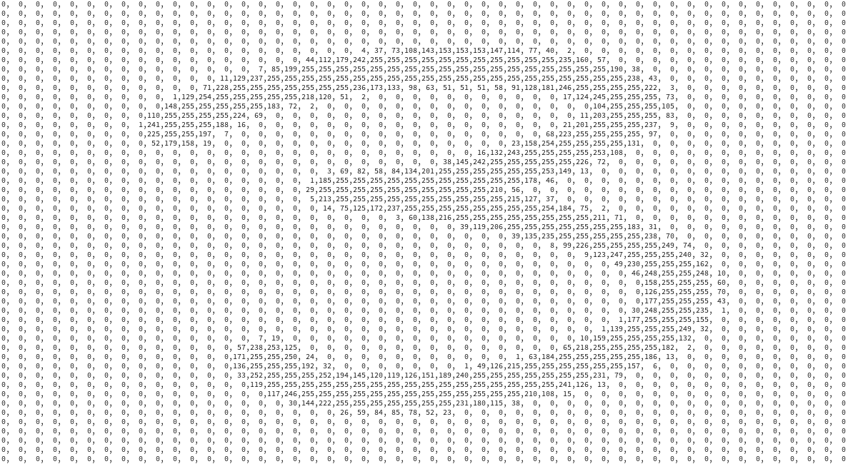
For a grayscale image, $X\in {\mathbb{R}}^{M\times N}$ where $M$ is the number pixels in the vertical direction, and $N$ is the number of pixels in the horizontal direction, and the intensity of the image pixels are represented as an 8-bit integer. Image below shows a [50px, 50px] hand-written digit that was converted to a grayscale image, where the numbers show the intensity of the given pixel.

Recall that the objective function in logistic regression applied to the classification problem was given by

$$\begin{array}{rl}f({\mathbf{w}}_1,\cdots ,{\mathbf{w}}_K)& :=-\sum _n\sum _k{t}_{nk}\log y_{nk}.\end{array}$$

Minimization of the objective function with respect to the weights requires, at minimum, evaluation of the first derivatives of the objective function (with respect to the weights). While this can be done by hand by repeated application of the chain rule, the common practice is to use back propagation on a graphical representation.

Figure below shows the equivalent graph of the network above for a single dataset.

In this graph, the evaluation of the objective function, $f$ begins at on the left-most end of the graph. The input data, $X$ (for a single dataset) is convolved with Layer 1 weights, $W^{(1)}$ producing $A^{(1)}$. This result is then passed on to the activation function, ${\sigma }_1$, convolved with Layer 2 weights, and so on.

Using the graph above as aid, the evaluation of the first gradient of the objective function with respect to layer weights starts at the opposite end of the graph, namely the right-most side.

Layer 3

Consider the evaluation of the derivative of the objective function, $f$, with respect to Layer 1 weights, namely $\frac{\partial f}{\partial W^{(1)}}$. Starting at the right-most part of the graph:

1. The right most portion $$\frac{\partial f}{\partial f}=1$$
2. Second element $$\frac{\partial }{\partial {\hat{y}}_p}\log {\hat{y}}_k\cdot t_k=t_p/y_p$$ (no sum)
3. Third from right $$\frac{\partial g(\sigma (z_k))}{\partial y_k}=\frac{\partial g(y_r)}{\partial y_p}\frac{\partial \sigma (z_p)}{\partial z_k}=t_k/y_k\cdot H(z_k)$$ (assuming ReLU activation function, no sum)
4. $$\frac{\partial }{\partial W_{pq}^{(1)}}g(W_{km}^{(1)}{v}_m)=\frac{\partial g(z_p)}{\partial z_k}\frac{\partial (W_{km}^{(1)}{v}_m)}{\partial W_{pq}^{(1)}}=t_p/y_{p}H(z_p)v_q$$

In the above $H(\cdot )$ is the Heaviside function.

The result of this process is shown in the graph below in color green.

Layer 2

1. $$\frac{\partial }{\partial v_p}g(W_{km}^{(1)}{v}_m)=\frac{\partial g(z_p)}{\partial z_k}\frac{\partial (W_{km}^{(1)}{v}_m)}{\partial v_q}=t_k/y_{k}H(z_k)W_{kq}^{(1)}$$
2. The 'Vec', which rearranges the contents of its argument can be reversed by rearranging a vector into appropriate shapes. Let this be denoted ${\hat{A}}_{pq}$
3. $$\frac{\partial g(\sigma (A^{(2)}))}{\partial {\hat{A}}_{km}^{(2)}}\frac{\partial {\hat{A}}_{km}^{(2)}}{\partial {\hat{A}}_{pq}^{(2)}}=H(A^{(2)}){\hat{A}}_{pq}$$ (Heaviside operator is understood as component-wise)
4. Convolution $$\begin{array}{rl}\frac{\partial }{\partial W_{pq}^{(2)}}g\left(Z^{(1)}\ast W^{(2)}\right)& =\frac{\partial g(A^{(2)})}{\partial A_{km}^{(2)}}\frac{\partial A_{km}^{(2)}}{\partial W_{pq}}\\ & =\frac{\partial g(A^{(2)})}{\partial A_{km}^{(2)}}\frac{\partial Z_{k-i,m-j}^{(1)}{W}_{ij}^{(2)}}{\partial W_{pq}}\\ & =H(A^{(2)}){\hat{A}}_{km}{Z}_{k-p,m-q}^{(1)}\\ & =\left(H(A^{(2)})\hat{A}\right)\star Z^{(1)}\end{array}$$ Where $\star$ denotes cross-corollation.

Layer 1

1. $$\begin{array}{rl}\frac{\partial }{\partial Z_{pq}^{(1)}}g\left(Z^{(1)}\ast W^{(2)}\right)& =\frac{\partial g(A^{(2)})}{\partial A_{km}^{(2)}}\frac{\partial A_{km}^{(2)}}{\partial Z_{pq}^{(1)}}\\ & =\frac{\partial g(A^{(2)})}{\partial A_{km}^{(2)}}\frac{\partial Z_{k-i,m-j}^{(1)}{W}_{ij}^{(2)}}{\partial Z_{pq}^{(1)}}\\ & =H(A^{(2)}){\hat{A}}_{i+p,j+q}{W}_{ij}^{(2)}\end{array}$$ (where valid, 0 otherwise)
2. $$\frac{\partial g({\sigma }_3(A^{(1)}))}{\partial A_{km}^{(1)}}\frac{\partial A_{km}^{(1)}}{\partial A_{pq}^{(1)}}=H(A^{(1)})H(A^{(2)}){\hat{A}}_{i+p,j+q}{W}_{i,j}^{(2)}$$
3. Convolution $$\begin{array}{rl}\frac{\partial g(A^{(1)})}{\partial W_{ij}^{(3)}}& =\frac{\partial g(A^{(1)})}{\partial A_{pq}^{(1)}}\frac{\partial X_{p-k,q-m}{W}_{km}^{(3)}}{\partial W_{ij}^{(3)}}\\ & =H(A^{(1)})H(A^{(2)}){\hat{A}}_{i+p,j+q}{W}_{i,j}^{(2)}{X}_{p-i,q-j}\end{array}$$

and $\tilde{A}:=H(A^{(1)})W_{pq}^{(3)}$ and $f\star g$ denotes the (discrete) cross-correlation of the two functions.

Summary

References

Suggested general reference books:

• Goodfellow, et. al Deep Learning (Adaptive Computation and Machine Learning series) . The MIT Press, 2016.

  Standard reference book on deep-learning. PDF copy is also available on author's webpage as of this writing.

• Bishop, Christopher M. Pattern Recognition and Machine Learning. Springer, 2006.

  Base reference for content of this page, though certainly not the best book that I have read.

• Boyd, Stephen, and Lieven Vandenberghe. Convex Optimization. Cambridge university press, 2004.

  A classic and a must-read introductory book to (convex) optimization for everyone regardless of their background. PDF copy is also available on Standford webpage as of this writing.

• Greenberg, Michael D. Foundations of Applied Mathematics. Courier Corporation, 2013.

  Good reference book or refresher on applied math.